Physically Grounded Monocular Depth
via Nanophotonic Wavefront Encoding

1 New York University2 Columbia University

* Equal contribution   † Corresponding authors

ECCV 2026
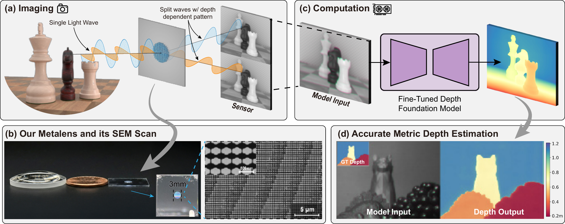
System overview: a birefringent metalens produces two polarization views; a fine-tuned depth foundation model recovers metric depth. The fabricated lens and nanopillars are shown below.
A single 3-mm metalens records two polarization views in one exposure (a). Depth-dependent shifts between the views provide a physical distance cue; a fine-tuned depth model combines it with learned scene structure to predict distance in metres (c–d). Panel (b) shows the fabricated lens beside a conventional lens and a coin, together with electron-microscope images of its nanopillars.

Overview

A birefringent metalens records two polarization images with depth-dependent point-spread functions (PSFs). We adapt a pretrained depth model to these image pairs and fine-tune it on simulated data and five real captures for single-shot metric depth estimation.

Video

Simulation Results

NYU Depth V2 · MPI Sintel · Hypersim · MIT-CGH-4K
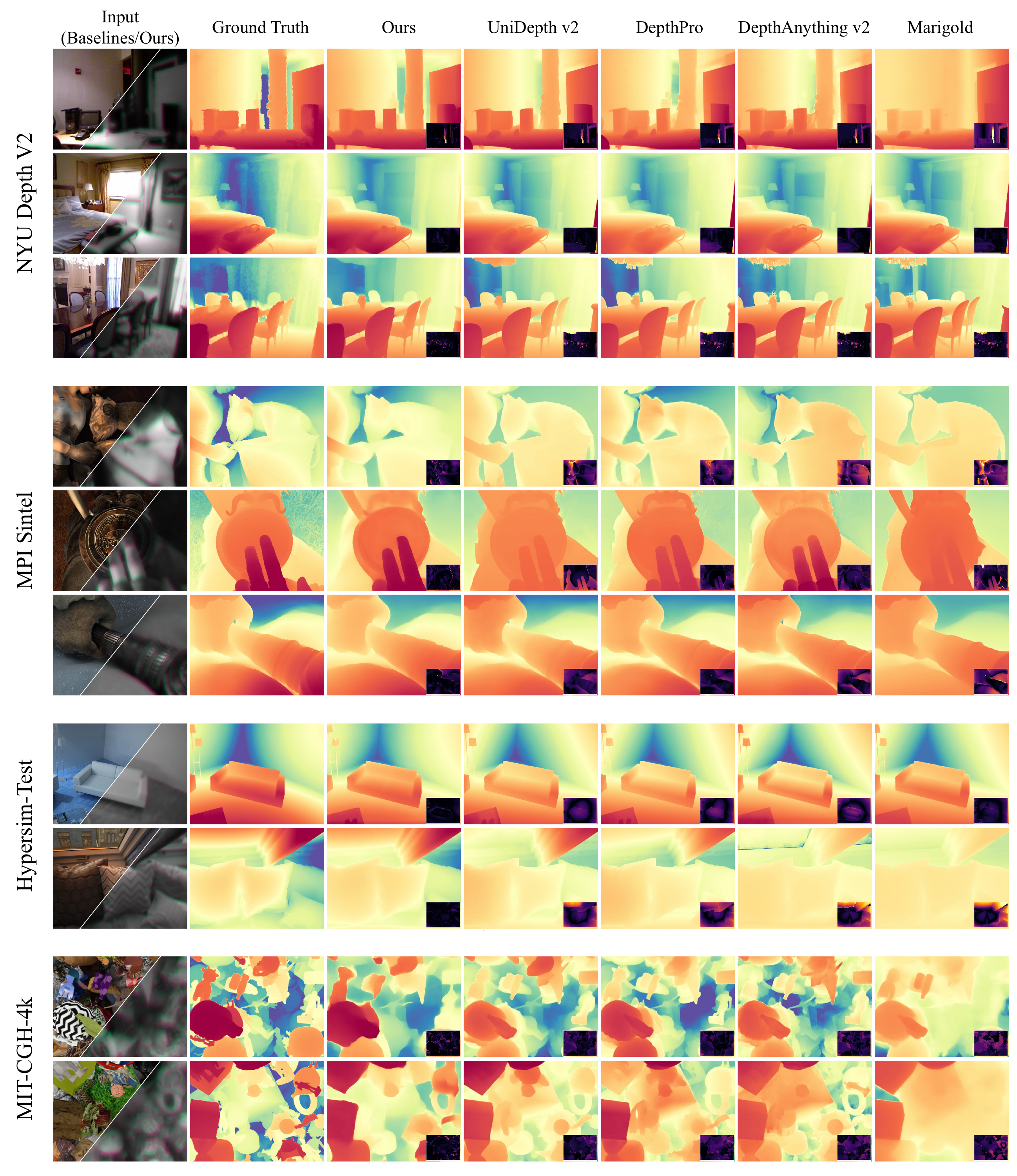
Ten simulated comparisons: three NYU Depth V2, three MPI Sintel, two Hypersim test, and two MIT-CGH-4K scenes. Columns show inputs, GT, ours, UniDepth V2, DepthPro, Depth Anything V2 and Marigold.
Each row compares one scene. The split input shows the baseline image (upper left) and our simulated polarization input (lower right), followed by ground truth and depth estimates. Warm colors indicate nearer surfaces; cool colors indicate farther ones. Darker error-map insets mean smaller errors. The cluttered MIT-CGH-4K examples show how physical depth cues help recover object distances when familiar scene context is weak. Baselines receive per-image scale-and-shift alignment to ground truth; our predictions are shown without this correction.

FlyingThings3D · Depth-prior ablation
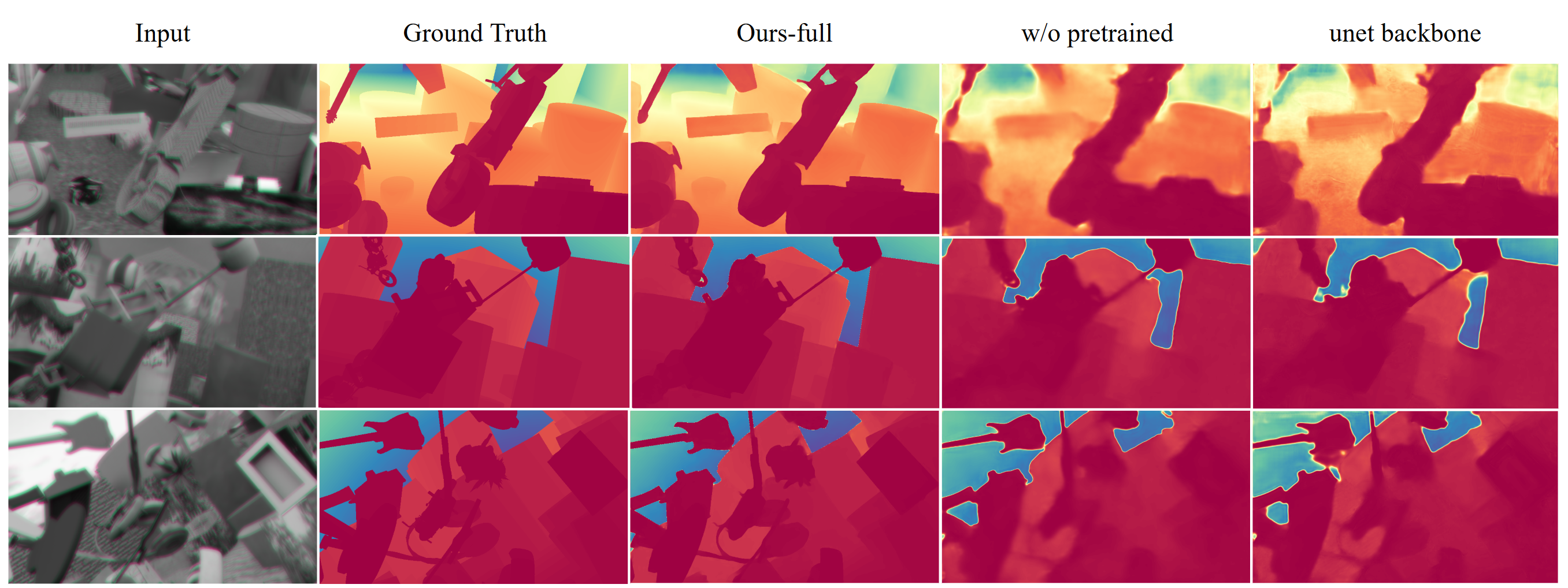
Three FlyingThings3D scenes comparing simulated inputs and ground truth with the full model, no pretrained initialization, and a U-Net backbone.
This ablation tests the contribution of pretrained depth priors. From left to right: simulated input, ground truth, our full model, the same architecture trained from scratch, and a U-Net alternative. Without pretraining, thin structures blur and surfaces lose their shape; the U-Net also introduces boundary and surface artifacts. The full model preserves these details more faithfully, showing the value of combining learned depth priors with optical cues.

Real Scenes

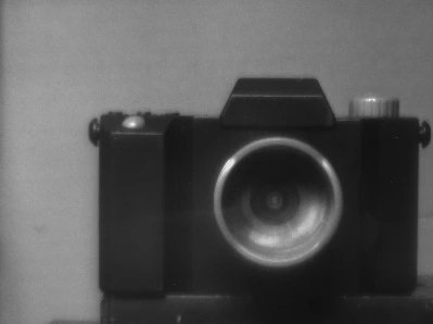
Polarization I₁: Camera
Polarization I₁
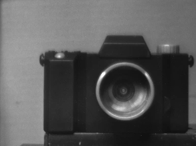
Polarization I₂: Camera
Polarization I₂
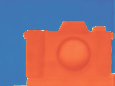
Ours · Large: Camera
Ours · Large
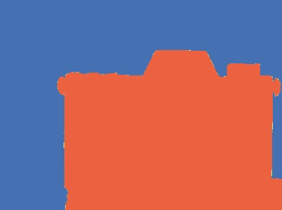
Depth labels: Camera
Depth labels
0.2 m1.2 m

3D View

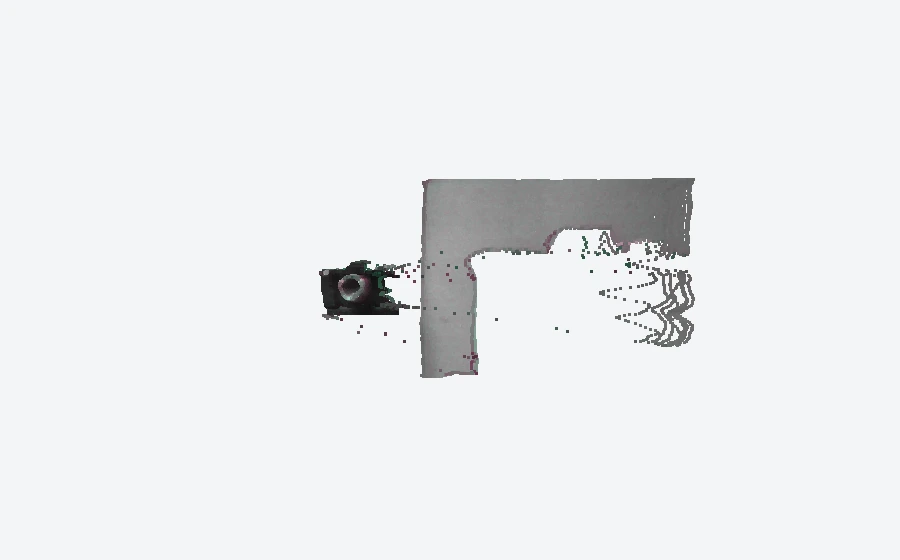
Rendered predicted point cloud: CameraSingle-view point cloud. The static preview is available from the scene thumbnails.Prediction preview · approximate projection
Loading interactive point cloud…

Real-World Comparisons

Single- and multi-object scenes captured with the prototype.
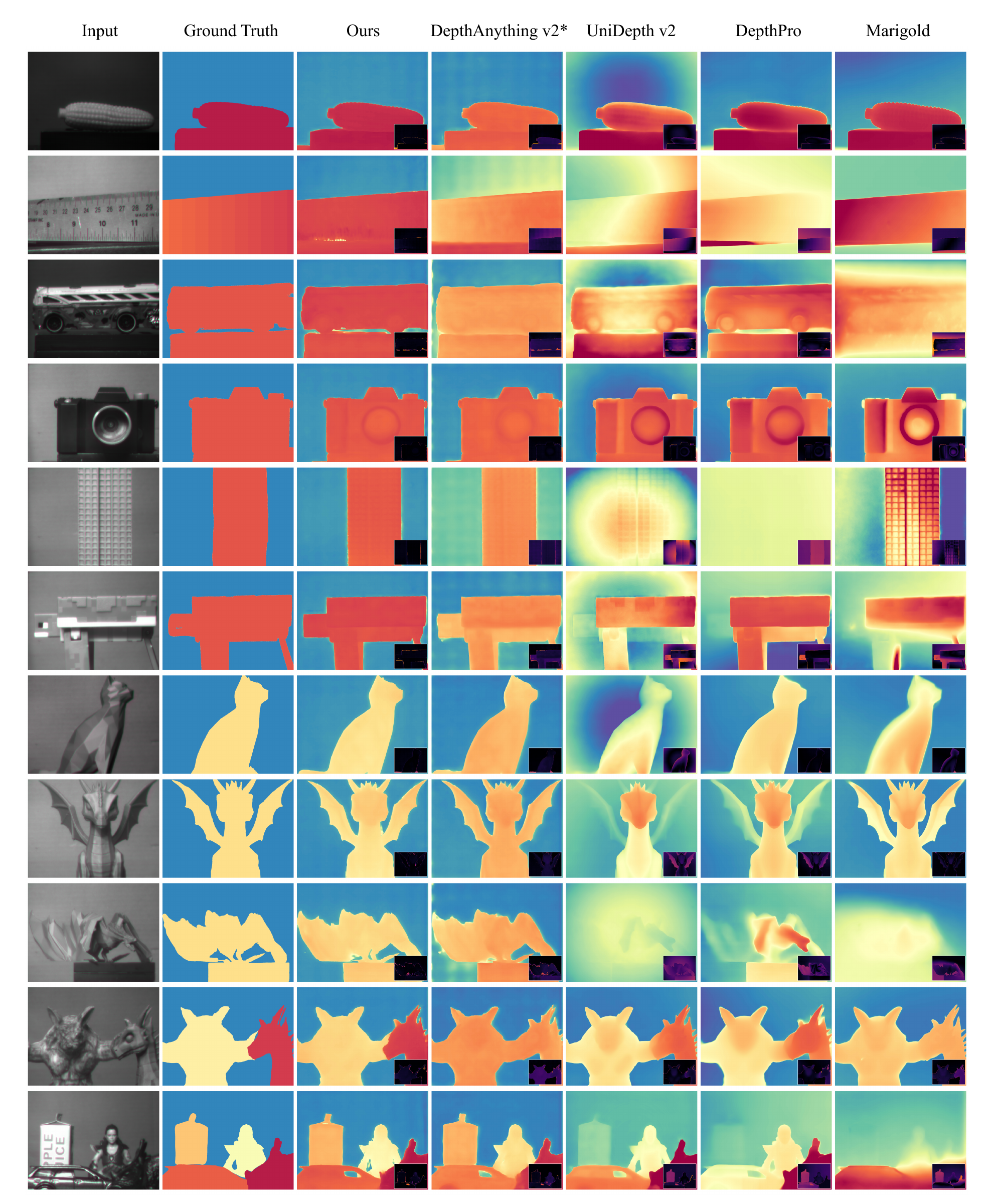
Eleven physical scenes comparing our paper results with Depth Anything V2, UniDepth V2, DepthPro and Marigold, alongside inputs and depth labels.
Eleven scenes captured with the metalens prototype, from single objects to objects at different distances. Compare both the object colors, which encode distance, and their boundaries with the reference labels. Our results preserve the separation between objects and background; darker error-map insets indicate smaller errors. Depth Anything V2* is fine-tuned without our depth encoding. It and our method are shown directly; other baselines receive scale-and-shift alignment to ground truth. Reference labels use measured object distances and manual masks, not dense surface scans.

Depth Consistency

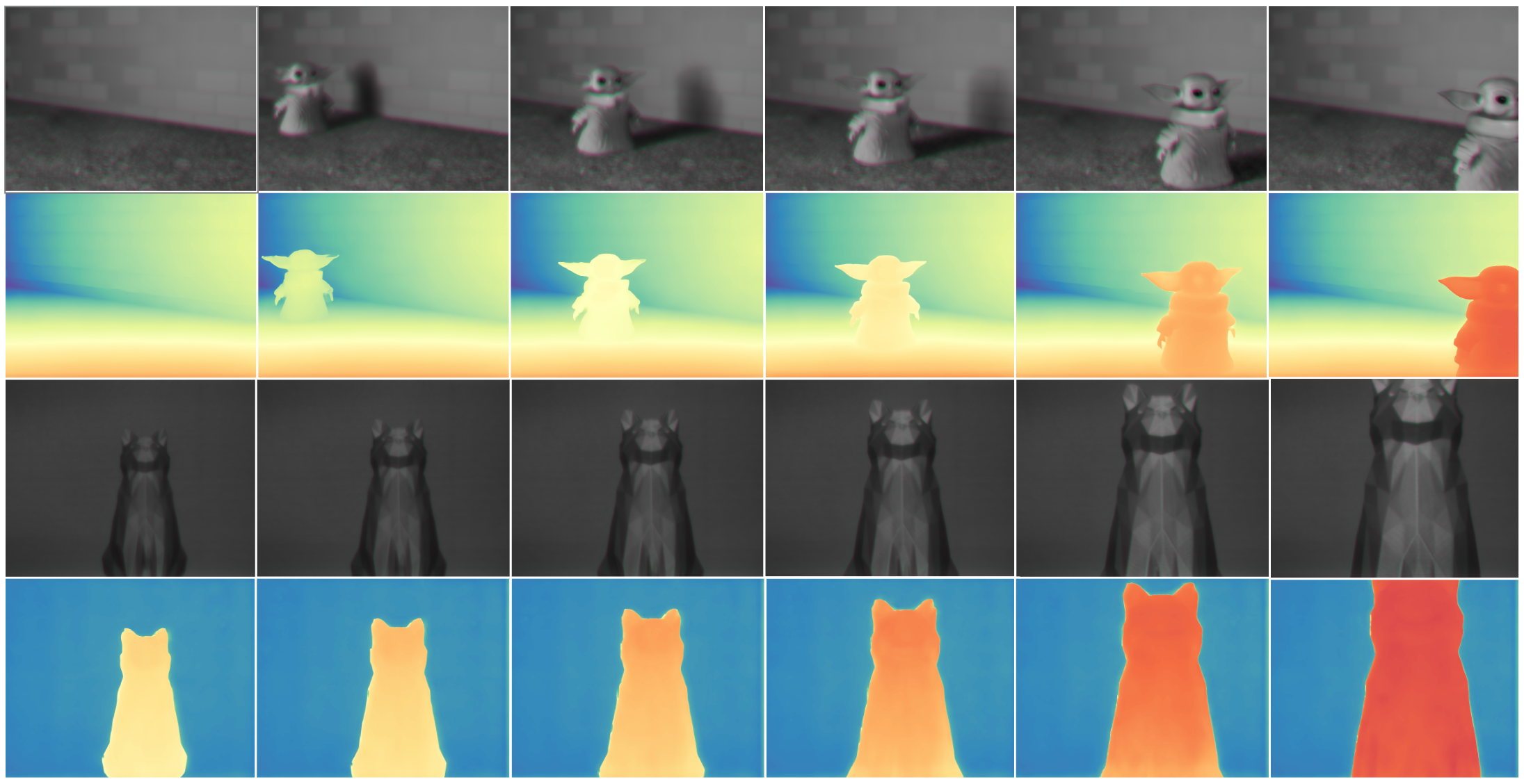
Six frames of input images and predicted depth: a simulated moving figure above and physical captures of a cat figurine moving toward the camera below.
Columns progress through time: a simulated moving figure is shown in the upper two rows, and a real cat figurine in the lower two. Each input row is followed by predicted depth. As the object approaches, its depth color changes from yellow toward orange and red while the background remains comparatively stable. These sequences illustrate consistent changes in estimated distance under motion.

Method

Our optical simulator maps RGB-D scenes to polarization image pairs. Both simulated and captured pairs are stacked as [Ix, Iy, (Ix + Iy) / 2] and passed to the depth model.
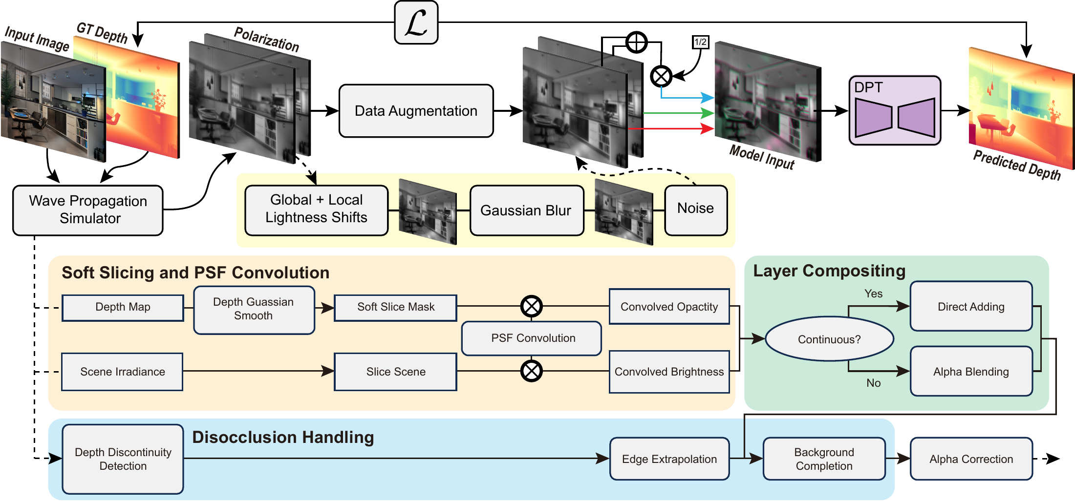
Full pipeline: RGB-D simulation, augmentation, three-channel input adaptation and depth prediction; the lower portion details the optical forward model.
The upper path turns RGB images and known depth into simulated polarization pairs. Brightness changes, blur, and noise approximate capture variations; the two views and their average form the three-channel input used to fine-tune Depth Anything V2. The lower path explains how the simulator combines depth layers and fills gaps near object boundaries. This supplies paired training data while reducing artifacts that would otherwise differ from real camera measurements.

Optical Simulation

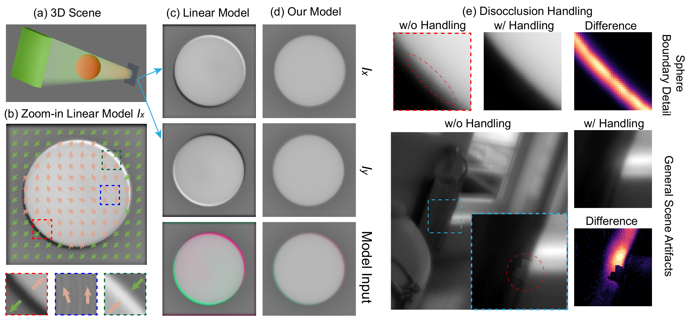
Linear convolution and our optical forward model, with sphere-boundary and indoor-scene ablations of disocclusion handling.
A foreground sphere exposes a problem with simple optical rendering: the linear simulator produces bright overlaps and dark gaps at object boundaries, plus sampling fringes on steep surfaces (b–c). Our simulator accounts for foreground–background visibility and fills newly exposed regions, reducing these artifacts (d). The sphere and indoor crops in (e) show what changes when this handling is enabled. This tests the quality of the training images generated by the simulator, not the depth network's predictions.

Polarization Robustness

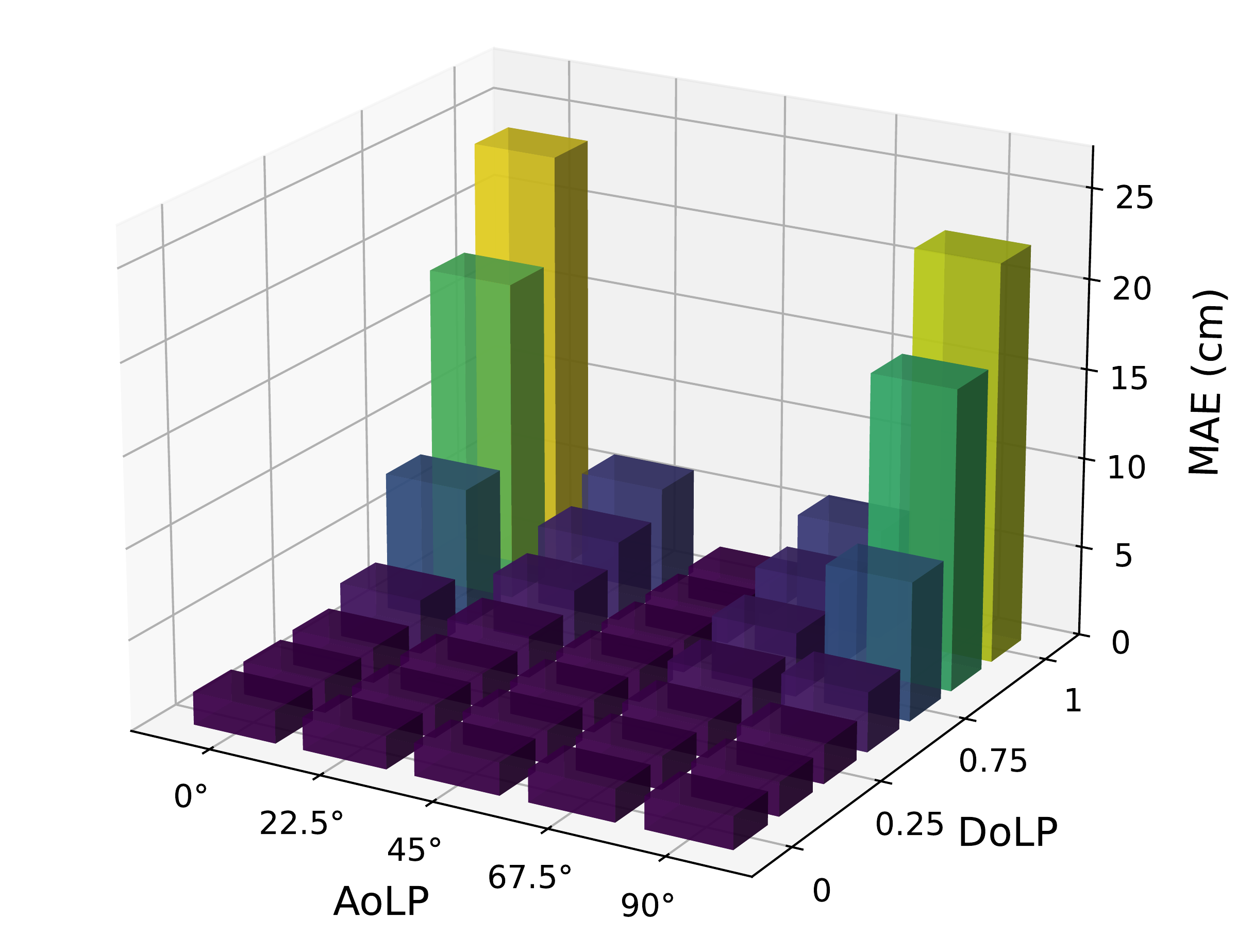
Hypersim depth error in centimeters as the degree and angle of linear polarization change.
Unequal brightness in the two polarization channels can weaken the depth cue. We simulate this on Hypersim by varying the degree of linear polarization (DoLP) and its angle (AoLP). Bar height shows mean absolute depth error in centimetres; lower is better. Error stays comparatively stable at moderate polarization, then rises at high DoLP, especially near 0° and 90°, where one channel becomes much dimmer. This tests global channel imbalance, not every form of spatially varying reflection or polarization.

Transfer to UniDepth V2

The same three-channel input adaptation with a different depth model.

Mean absolute depth error (MAE), in metres; lower is better. Fine-tuning the Small UniDepth V2 model on our polarization input gives lower error than the original Large model on all three datasets. This shows that the input adaptation also works with a second depth-model family, rather than depending only on Depth Anything V2. Results are reproduced from the supplementary material.
DatasetOriginal LargeFine-tuned Small
NYU Depth V20.03380.0217
MIT-CGH-4K0.12730.0708
Real captures0.10680.0348

PSF Analysis

A point-spread function (PSF) is the image formed by a point of light. Our design makes it rotate with distance and records opposite lobes in separate polarization channels. These theoretical comparisons use a 1–5 m range and 50 mm focal length, not the near-range prototype.

Point Sources and Photon Budget
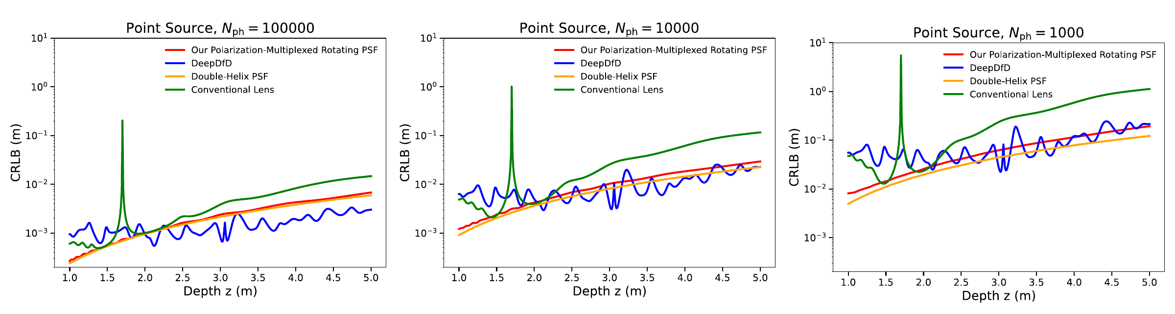
Depth precision bounds for our PSF, DeepDfD, double-helix and conventional lens designs at three photon budgets.
A point of light is imaged at different distances with four PSF designs. The vertical axis is the Cramér–Rao bound (CRLB): a theoretical lower limit on the standard deviation of an unbiased depth estimate, not measured model error. Lower values on this logarithmic axis mean better attainable precision. From left to right, the photon budget falls from 100,000 to 10,000 to 1,000. The rotating designs avoid the conventional lens’s near-focus spike and vary smoothly with depth; DeepDfD’s relative performance depends on distance and photon budget.

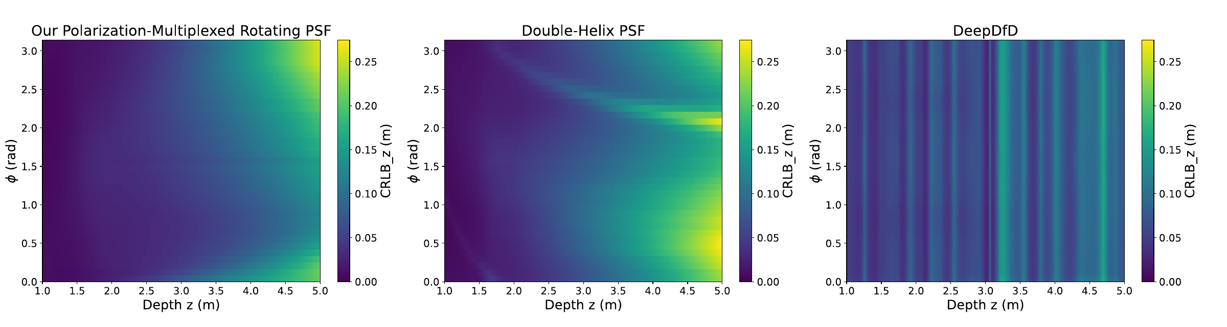
Edge Orientation

Heatmaps of the depth precision bound versus distance and edge orientation for our PSF, double-helix and DeepDfD designs.
A straight bright–dark edge models an object boundary. The horizontal axis is its distance and the vertical axis its orientation in radians; both are unknown in this calculation. Purple means a lower depth-uncertainty bound, yellow a higher one. Our polarization-separated rotating PSF varies smoothly across orientations, whereas the double-helix design has pronounced bands of poorer precision. Separating the lobes therefore reduces this orientation-dependent ambiguity. DeepDfD is nearly orientation-independent because its PSF is radially symmetric.

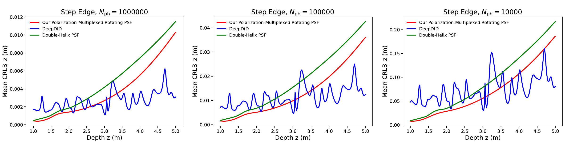
Extended Edges and Photon Budget

Orientation-averaged edge depth precision bounds at three photon budgets for three PSF designs.
These curves average the edge depth-uncertainty bound over orientation. Lower is better. From left to right, the photon budgets are one million, 100,000, and 10,000; each panel has a different vertical scale. Our design (red) has a lower mean bound than the double-helix PSF (green) throughout the plotted range, supporting the benefit of separating its two lobes into polarization channels. The comparison with DeepDfD (blue) depends on depth and photon budget; no design is best everywhere.

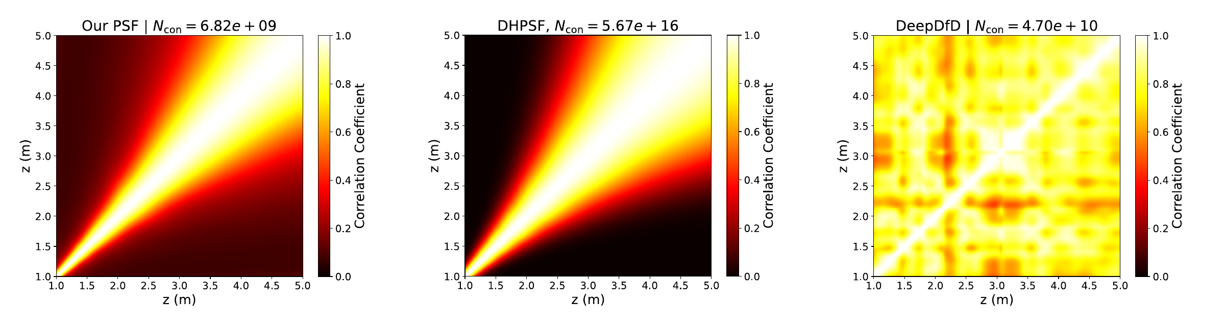
Ambiguity Across Depths

Pairwise PSF correlation matrices over one to five meters for our PSF, double-helix and DeepDfD designs.
Each pixel compares the PSFs at two distances, read from the horizontal and vertical axes. Yellow and white mean high similarity; bright regions away from the diagonal indicate depths that can be confused. Both rotating designs concentrate similarity near the diagonal, unlike DeepDfD’s broadly similar patterns. The reported condition number describes how sensitive optical depth recovery is to measurement errors. Ours is about one-seventh of DeepDfD’s, supporting more stable recovery in this theoretical setting.

Resources

Code includes the optical simulator, training, and inference. Checkpoints are available in Small, Base, and Large sizes. The dataset contains five training scenes and 42 evaluation scenes. Inputs and depth labels are available under CC BY-NC 4.0 for noncommercial use, including academic research.

Evaluation protocol and limitations

The 42 scenes were also used for validation and model selection, not as an untouched holdout. Their depth labels are manually segmented regions assigned measured object distances, not dense 3D scans. The explorer uses the selected mixed-training Large checkpoint; paper figures retain their original results and are not a fresh benchmark.

The prototype targets well-lit, near-range scenes. Limited light throughput, field of view, and high-frequency polarization imbalance remain limitations. Code is MIT-licensed with retained third-party notices. Small weights follow Apache-2.0; Base and Large follow CC-BY-NC-4.0.

BibTeX

@article{li2026physically,
  title={Physically Grounded Monocular Depth via
         Nanophotonic Wavefront Encoding},
  author={Li, Bingxuan and Wu, Jiahao and Xu, Yuan and
          Zhu, Zezheng and Zhang, Yunxiang and Chen, Kenneth and
          Liang, Yanqi and Yu, Nanfang and Sun, Qi},
  journal={arXiv preprint arXiv:2503.15770},
  year={2026}
}